First things first: what is probability?

Probability is a measure or estimate of how likely a certain event is to happen. Another way to put it: how likely a statement is to be true.

Probability theory is the branch of mathematics concerned with these measurements and estimations. It’s a relatively new branch (when compared to algebra or calculus, for instance), but it’s gaining a lot of importance in recent years, with applications in medical sciences, computer sciences, artificial intelligence, big data and so on.

Below you’ll find an introduction on the subject that aims to cover all the core probability principles, explaining them with examples and in a manner (hopefully) easy to understand.

Definitions and Terminology

Experiment: A process leading to two or more outcomes, where there’s some uncertainty regarding which outcome will take place. An experiment could be tracking the price of a stock, rolling a couple of dice, or asking the name of the next person that will come by in the street, for instance. Sometimes also called “random experiment”.

Sample space: The set of all the possible outcomes of an experiment is called the sample space. If your experiment is rolling a die, for instance, your sample space would be S = {1,2,3,4,5,6}. If you toss a coin, your sample space would be S = {Head,Tail}.

Event: An event is any subset of the sample space. The event is said to take place if the experiment generates one of the outcomes that is part of the event’s subset.

With those definitions out of the way, we can start talking about probability. First of all probability is expressed with numbers between 0 (representing 0% chance of happening) and 1 (representing 100% chance of happening). This makes the first postulate of probability:

Postulate 1: The probability of any event must be greater than or equal to 0, and smaller than or equal to 1. So 0 ≤ p ≤ 1

Since the sample space is composed of all the possible outcomes, when you run an experiment, one of those possible outcomes will necessarily occur. This means that the combined probability of all possible outcomes must be 100%, and that’s the second postulate:

Postulate 2: The sum of the individual probabilities of all the outcomes in the sample space must always be equal to 1. So ΣP(e) = 1.

That’s it. The above definitions and postulates are pretty much all you need to have a formal way of working with probability.

Probability is Counting

If you think about it, measuring probability is basically a matter of counting things. On one hand you have the sample space, which is the finite set of all the possible outcomes. On the other hand you have an event, which is a certain subset of outcomes of the sample space. The probability that the event will take place is the number of outcomes that lead to the event divided by the total number of possible outcomes. This is the classic definition of probability.

Let’s use some numerical examples.

What’s the probability of getting a 6 when you roll a die?

The sample space is S = {1,2,3,4,5,6}, and the event we are interested is the 6 showing up. So the probability of getting a 6 is 1/6 or 0.166 (0.166 is equivalent to writing 16,6%).

Now let’s do something slightly more complex. Suppose you’ll toss two coins in a row. What’s the probability of the following events (please take a moment and try to estimate the probabilities, either in your head or with pen and paper):

A: Tossing two heads in a row
B: Tossing at least one head
C: Tossing exactly one head and one tail (the order doesn’t matter)

As you’ll see later on this article, one could use probability rules and equations to find the probability of these events. However, if you understand how to count things the correct way, you can solve it easily.

And here comes a tip: when trying to find probabilities via the counting method, always start with writing down your sample space. In our case, there are 4 possible outcomes:

1st Coin  -  2nd Coin
Head      -  Head
Head      -  Tail
Tail      -  Head
Tail      -  Tail

You can see that event A requires 1 out of 4 possible outcomes, so its chance is 1/4 or 25%. If the chance of tossing two heads in a row is 25%, we can conclude that the probability tossing two tails in a row is also 25%, due to the symmetry of the experiment.

Event B has 3 out of 4 possible outcomes, so its chance is 3/4 or 75% (which makes sense, cause the probability of tossing at least one head should be equal to one minus the probability of tossing two tails, which is 25% as we saw above).

Finally, event C has 2 out of 4 possible outcomes, so a 50% chance of happening.

Probability and Set Theory

As you have seen above, probability theory shares many principles with set theory (the branch of mathematics concerned with sets). Below you’ll find principles and definitions that solidify even more this relationship. In fact in each case we’ll be using a Venn Diagram (a diagram that shows all possible relations between a collection of sets) to illustrate what’s going on.

Complement of an Event: The complement of an event is the subset of outcomes that belong to the sample space but that do not belong to the event itself. In other words, all the outcomes that don’t satisfy the event itself.

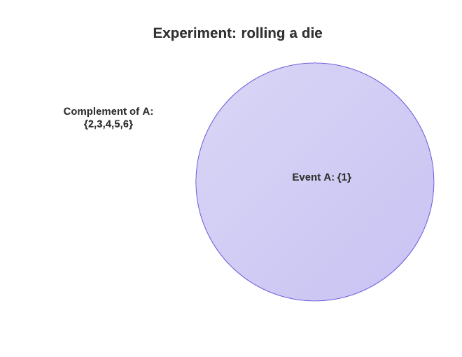
Example: Say we are rolling a die and event A is getting a 1. The complement of event A would be not getting a 1, therefore getting either a 2, 3, 4, 5 or 6. The probability of event A is 1/6, and the probability of the complement of event A is 5/6. You can arrive at the 5/6 either by adding the individual probabilities of all the outcomes that don’t belong to A, or by simply doing 1 – P(A) (i.e., 1 – 1/6 = 5/6).

Union of Events: The union of two or more events is the subset of outcomes that belong to at least one of those events. Union of events A and B is denoted by A∪B. In other words, if you are interested in the union of events A and B you are interested in either event A OR event B happening (or both).

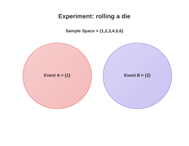
Example: Suppose that you will roll a die. Event A is a 1 showing up. Event B is a 2 showing. This experiment is illustrate in the Venn Diagram above.

The union of those events is either a 1 OR a 2 showing up. As you noticed, when we talk about union of events, we are talking about one event OR the other, and when you want to find the probability of the union of two events you need to ADD their individual probabilities (there’s a special case, but I’ll explain it later on).

Therefore P(A) = 1/6, P(B) = 1/6, and P(A∪B) = 1/6 + 1/6 = 2/6.

Another way of putting it: you have one event with probability 1/6 of happening, and another event with probability of 1/6 as well. If you are interested in either one or the other happening, you are basically combining their individual probabilities, that’s why you add them together.

You can also use the counting method to arrive at the same result. There are 6 possible outcomes, and 2 of those satisfy the union of events A and B, so the probability of the union is 2/6.

And this gives us our first rule:

Rule 1: When considering the union of events (i.e., one event OR the other) you need to add their individual probabilities to find the probability of the union.

Intersection of Events: The intersection or two or more events is the subset of outcomes that belong to all the events. Intersection of events A and B is denoted by A∩B. In other words, if you are interested in the intersection of two events you want to know the outcomes that will satisfy both events at the same time.

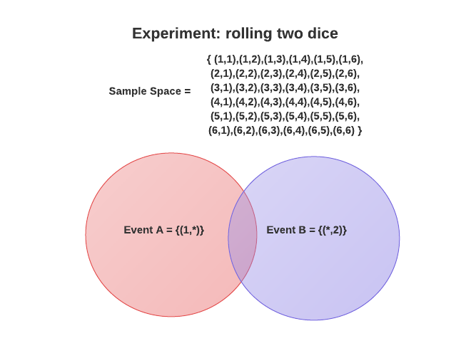
Example: Suppose that you will roll two dice now. The sample space of this experiment has 36 possible outcomes, as you can see on the Venn diagram above. Outcome (1,1) represents a 1 showing up on both dice. (1,2) represents a 1 showing up on the first die and a 2 on the second. So on and so forth. There are 36 possible outcomes because you have 6 possibilities on the first die and 6 on the second, so 6 * 6 = 36.

Now let’s say that event A is getting a 1 in the first die (and therefore anything on the second die), so (1,*). Event B is a 2 showing up in the second die (and therefore anything on the first die), so (*,2). The intersection of those events is a 1 showing up in the first die AND a 3 showing up in the second die. The intersection in the Venn diagram is the section where the two circles overlap.

Getting a 1 on a die has the probability of 1/6, so that’s the probability of event A. We could also use the counting method with the whole sample space. There are 36 possible outcomes rolling the two dice, and 6 of those satisfy event A (i.e., the six where there’s a 1 in the first die). So 6/36 = 1/6.

The sample thing applies to event B, to P(B) = 1/6.

Now what’s the probability of the intersection, P(A∩B)?

Let’s use the counting method again. There are 36 total possible outcomes. Out of those only one will satisfy the intersection of events A and B, and that is getting a 1 on the first die and a 2 on the second, so (1,2). In other words, P(A∩B) = 1/36.

Another way of arriving at this result is by multiplying together the individual probabilities. 1/6 * 1/6 = 1/36. And this gives us our second rule:

Rule 2: When considering the intersection of events (i.e., one event AND the other) you need to multiply the individual probabilities to find the probability of the intersection. (This is true only for independent events, but I'll talk about those later on).

Notice that we could have an event C defined as follows: the sum of the numbers appearing on the two dice is equal to 3. The probability of this event would be 2/36 because there are 2 outcomes out of 36 that would satisfy this event: (1,2) and (2,1).

Mutually Exclusive Events: if in the sample space there are no outcomes that satisfy events A and B at the same time we say that they are mutually exclusive. In other words, either event A happens, or event B, but not both.

Example: The first consequence of having mutually exclusive events is that they won’t have an intersection (formally speaking their intersection will be the empty set). One example of mutually exclusive events is this: the experiment is rolling a die, event A is getting a 1 and event B is getting a 2. Clearly either one event will happen or the other, so they are mutually exclusive. You can see this graphically on the Venn diagram used for our union example above.

The second consequence is related to events that ARE NOT mutually exclusive. Those events will have an intersection, and when trying to calculate the probability of the union of those events you need add their individual probabilities together AND subtract the probability of their intersection (else you would be counting some outcomes twice). We therefore need to revise our first rule:

Rule 1 Revised (called the "addition rule"): P(A∪B) = P(A) + P(B) - P(A∩B)

Notice that the above rule/equation is valid for non mutually exclusive events as well as for mutually exclusive ones. That’s because if the events are mutually exclusive P(A∩B) = 0, so the equation will become P(A∪B) = P(A) + P(B) anyway. If the events aren’t mutually exclusive, on the other hand, then subtracting their intersection will produce the correct result.

Notice also that you can move the terms around, like this:

P(A∩B) = P(A) + P(B) - P(A∪B)

Meaning that if you know the individual probabilities of the events and their intersection you can calculate their union, and if you know the union you can calculate their intersection.

Example: Let’s consider the experiment of rolling two dice (the same we used to show the intersection of two events above). Again let’s say that event A is getting a 1 in the first die, and event B is getting a 2 in the second die. Those events are clearly not mutually exclusive, there’s at least one outcome that satisfy both at the same time. How do we calculate the union of those events then? That is, what’s the probability that when rolling two dice you’ll get either a 1 on the first die OR a 2 on the second die?

First of all remember that the individual probabilities of each event is 1/6, so P(A) = 1/6 and P(B) = 1/6. Someone who is not aware of the addition rule could say that the union of those two events is simply P(A) + P(B), which is equal to 2/6, but this is not the correct probability, because you are counting the outcome where both events happen (i.e., their intersection) twice. Let me show with the numbers:

The following outcomes satisfy event A: (1,1), (1,2), (1,3), (1,4), (1,5), (1,6)
The following outcomes satisfy event B: (1,2), (2,2), (3,2), (4,2), (5,2), (6,2)

The union of those events is the subset of events that satisfy both, so all the outcomes listed above, without repetitions. The outcome (1,2) appears on both lines, so you need to count it only once.

The outcomes that form the union of A and B therefore are: (1,1), (1,2), (1,3), (1,4), (1,5), (1,6), (2,2), (3,2), (4,2), (5,2), (6,2)

As you can see there are 11 outcomes, so the probability of the union is 11/36, which is not equal to 2/6.

We can arrive at the same result using the equation of rule 1.

P(A∪B) = P(A) + P(B) - P(A∩B)

Remember that P(A∩B), the probability of the intersection of events A and B, is 1/36. So:

P(A∪B) = 1/6 + 1/6 - 1/36 = 6/36 + 6/36 - 1/36 = 11/36

Conditional Probability

Conditional probability is concerned with finding the probability of event A GIVEN that event B already happened. Another way of putting it: the probability of event A with the CONDITION that event B already happened. That is, we know for sure that B happened, and now we want to find the probability of A given this information we have.

The first thing you should notice is that the conditional probability of mutually exclusive events is always zero. Let’s use our favorite example: the experiment is rolling a die, event A is getting a 1, event B is getting a 2. What’s the probability of A given that the die showed a 2? It’s clearly zero (i.e., if the die showed a 2 it certainly didn’t show a 1, so the probability of A is 0%).

This implies that most of the time when we talk about conditional probability we’ll be talking about non-mutually exclusive events.

That being said, here’s how you calculate conditional probability: the probability that event A happens given event B already happened is the probability of both events happening (i.e., their intersection) divided by the probability of event B.

An easier way to understand this is the following: the probability that event A happens given event B already happened is the number of outcomes that satisfy both A and B, divided by the total number of outcomes that satisfy B. That is, you are trying to find the number of times that when B happens A will happen as well. If 50% of the time B happens A will happen as well, then you know that the probability of A given B is 50%.

Probability of A given B is written as P(A|B), and our rule 3 is:

Rule 3 (conditional probability): P(A|B) =  P(A∩B) / P(B)

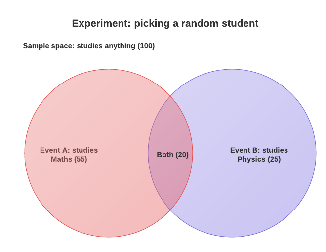
Example: The Venn diagram above illustrates this example. Suppose we have a school with 100 students, and our experiment is picking one student at random. Event A is that the picked student studies math. Event B is that the picked student studies physics.

We know that 55 students in the school study math, 25 study physics, and 20 study both subjects. And just to be clear, by “55 students study math” we don’t mean that they study ONLY math. We mean that 55 students study math, and some of those 55 might as well study other subjects, including physics (in fact we know that 20 of them do study physics as well).

We obviously know that P(A) = 55/100, P(B) = 25/100 and P(A∩B) = 20/100. Now suppose we pick a student at random, and he does study physics. What’s the probability that he also studies math? This is basically the conditional probability of A given B, or P(A|B).

P(A|B) = P(A∩B) / P(B) = 20 / 25 = 0.8

So if we pick a random student and he studies physics, the probability that he also studies math is 80%. Another way of saying this is that 80% of the students who study physics also study math.

We can easily invert this. The probability that a student studies physics given he studies math is:

P(B|A) = P(A∩B) / P(A) = 20 / 55 = 0.36

So given a students studies math he has a probability of 36% of studying physics too.

Notice that you can also move the terms of the conditional probability rule around, getting a variation, which is called the “multiplication rule”.

Variation of rule 3: P(A∩B) = P(A|B) * P(B)

Statistical Independence of Events

Two events are said to be statistically independent, or simply independent, if the occurrence (or non-occurrence) of one event does not affect the probability of the other event. In other words, if events A and B are independent, the conditional probability of event A given event B is the same as the probability of event A. So:

P(A|B) = P(A) 
P(B|A) = P(B)

If you plug this into the multiplication rule you get:

P(A∩B) = P(A|B) * P(B)

so:

P(A∩B) = (PA) * P(B)

And this is another way of defining statistical independence. If events A and B are independent then the probability of their intersection is equal to the multiplication of their individual probabilities.

Notice that you can’t know whether two or more events are independent of each other by solely analyzing their description. You need to actually analyse the probabilities involved to be sure.

And here’s a point where many people get confused: by definition, mutually exclusive events can never be statistically independent, because their intersection is always equal to zero. That is, if P(A|B) = 0, P(A|B) can’t be equal to P(A).

The only exception to this is the case where the probability of either event A or B is equal to zero. If P(A) is zero then events A and B can be mutually exclusive and independent at the same time, because P(A|B) = (PA) = 0, and P(A∩B) = (PA) * P(B) = 0.

A real life example of this exception would be the following: the experiment is rolling a die. Event A is getting a 7, and event B is getting a 3. P(A) = 0, P(B) = 1/6, P(A|B) = 0, P(A∩B) = 0, therefore the events are both mutually exclusive and independent.

To illustrate the concept of statistical independence let’s consider again the experiment of rolling two dice, where event A is getting a 1 in the first die and event B is getting a 2 in the second die, as describe in the Venn diagram below:

Are events A and B independent? Let’s investigate:

P(A) = 1/6
P(B) = 1/6
P(A∩B) = P(A) * P(B) = 1/6 * 1/6 = 1/36

So yeah the events are independent. You can also confirm this via the conditional probability rule.

P(A|B) = P(A∩B) / P(B) = 1/36 / 1/6 = 6/36 = 1/6 = P(A)

In other words, when running this experiment, the fact that the first die shows (or doesn’t show) a 1 doesn’t affect the probability of the second die showing a 2, and vice-versa, so the events are statically independent.

And whether the events are independent or not you can always use the addition rule to calculate their intersection. So:

P(A∩B) = P(A) + P(B) - P(A∪B)

Remember that the union of these events is 11/36, so:

P(A∩B) = 1/6 + 1/6 - 11/36 = 6/36 + 6/36 - 11/36 = 1/36

Now let’s consider the example of the students again, as describe by the Venn diagram below:

Remember that event A is the student studs math, and event B is the student studies Physics. Are those independent?

P(A) = 55/100
P(B) = 25/100
P(A∩B) = 20/100

If the events were independent then their intersection should be equal to the multiplication of their individual probabilities.

P(A∩B) = P(A)*P(B) = 55/100 * 25/100 = 1375 / 10000 (so not equal to 20/100)

As you can see the results are not the same, so the events are dependent. Another way of seeing it: if you pick a student at random, his chance of studying math is 55%. If you pick a student at random and discovers he studies physics (i.e., event B happened), however, then the chance that this student also studies math is now 80%, which is greater than before. So the occurrence of one event affects the probability of the other happening, and thus the events are dependent.

Again let’s use the addition rule to confirm the results. First we need to find the union of these two events. P(A∪B) = 60/100, so:

P(A∩B) = 55/100 + 25/100 - 60/100 = 20/100

Independence of 3 or More Events

If you have 3 or more events, the individual pairs of events might be independent between them, but that doesn’t mean all events will be independent at the same time.

For instance, suppose a computer will randomly print the strings “a”, “b”, “c” and “abc” with equal chance. Each pair of events is independent between themselves, but all the events together are not. (Example from Harvard Prof. Paul Bamberg).

P(a) = 1/2 (probably that an ‘a’ will be printed is 1/2, cause it can be printed individually or inside ‘abc’).
P(b) = 1/2
P(c) = 1/2
P(abc) = 1/4

Now P(a∩b) = 1/4 = P(a)P(b), so this shows this pair of events is independent.
Same is valid for P(a∩c) and P(b∩c).

However, P(a∩b∩c) = 1/4, which is different from P(a)P(b)P(c) = 1/8, so these three events are not independent.

Here’s how to view it in words. For events to be independent the occurrence of one should not affect the probability of the other taking place. This is not true for the 3 events, because once you know that both ‘a’ and ‘b’ were printed you know for sure that ‘c’ was also printed, so the occurrence of the first two affects the probability of the third taking place.

Permutations and Combinations

Permutations and combinations are not actually part of the probability theory (they are part of a mathematics branch called combinatorics). However, as we have seen probability is about counting, and often time you’ll need to use permutations and/or combinations to calculate the total number of outcomes on a given experiment.

Permutations refer to the different sequences in you can make with a group of objects. In other words, it refers to the different orders in which you can arrange the objects. The key point is that ordering matters in permutations.

Suppose you have the letters a,b,c, and e. How many permutations there are of those 4 letters? Basically you have 4 options when choosing the first letter, 3 when choosing the second, 2 when choosing the third and only one option when choosing the last letter. So there 4x3x2x1 = 24 total permutations.

As you probably noticed this is equal to 4!. So if you have N objects, there are N! permutations of those objects.

What if we have the same four letters, but we only want to print two of them at time. How many permutations are there now? Basically the permutations now are: ‘ab’, ‘ac’,’ad’,’ba’,’bc,’bd’,’ca,’cb,’,’cd’,’da’,’db’,’dc’. So there are 12 permutations.

This is basically 4! / 2!. The general case is that if you have N objects and want to permutate K at a time then the total number of permutations is

Number of permutations of N elements, use K at a time =  N! / (N-K)!

This formula can be applied even to the case where you have N objects and permutate N at a time, because 0! = 1, so N! / (N-N)! = N!:

Combinations, on the other hand, refer to the number of different subsets of a given set. In other words, the order of elements doesn’t matter here. For instance, if our set is the same four letters are before (i.e., ‘abcd’), then the subset ‘abc’ is the same as the subset ‘acb’ or ‘cba’.

So how many combinations of four letters are there if our set is {a,b,c,d}?

Only one, since there is only one way to choose 4 letters out of a set with 4 letters.

Now how many combinations of three letters are there of the set same?

Four: ‘abc’, ‘abd’, ‘acd’,’bcd’.

How many combinations of two letters?

Six: ‘ab’, ‘ac’, ‘ad’,’bc’,’bd’,’cd’.

Say we have a set with N elements and want to choose K of those. The number of combinations can be found by using the same formula of permutations, except that now you need to divide the result by K!, to if we didn’t we would counting same subsets with different order. By dividing by K! we are basically saying that the order doesn’t matter. So the formula for combinations become:

Number of combinations of N elements choose K at a time = N! / K! (N-K)!

Example: Consider that our experiment is dealing 5 cards out of a normal 52-card deck. What’s the probability of getting four cards of the same kind (i.e., 4 aces or 4 kings) in that hand?

We could solve this problem by finding first how many different ways there are of picking 5 cards out of 52. The answer is:

52!/47!5! = 52*51*50*49*48 / *5*4*3*2*1 = 2,598,960

Now how many of those 5-card combinations would contain 4 cards of the same type? To makes things easier let’s break the problem down and first find the number of combinations where we would have 4 aces specifically (we picked aces, but it could be any card, since there’s the same number of each on the deck).

Another way of putting it, how many ways can we build a hand with 5 cards where 4 of those are aces?

We basically need to put 4 aces there (no choice here) and the fifth card can be any of the remaining 48 cards (so 48 choices). So there are 48 combinations where we have 4 aces (remember that the order of the cards doesn’t matter here, so we are talking about combinations and not permutations).

Now there are 13 types of cards in a deck, so the number of combinations with four repeat cards of any kind on our 5-card hand is 13 * 48 = 624.

Finally, the probability of getting 4 cards of the same kind on a 5-card hand is therefore 624 / 2,598,960, which is equal to 2,4%.